Original post date: January 3, 2026
Wavetable synthesis
Steps
You can try playing around with the steps, or you can instantly try an example where I'm saying "Kai Saksela" by pre-filling it with some example data .
Load a WAV file
A WAV file is basically a header plus PCM sample data. We decode it into a normalized floating-point signal.
Step 1
Load a WAV file
We load a .wav file into memory. Nothing is sent to a server; all processing is done in the browser.
Visualize the waveform
This view is mostly for sanity-checking: it helps confirm the file decoded correctly and whether it looks OK.
Step 2
Visualize the waveform
After simple preprocessing (convert the signal to mono, remove silence), plot what the waveform looks like.
Waveform
Load a WAV file to see its waveform.
Compute YIN / CMNDF heatmap
There are many ways to assess periodicity of a signal varying in time. The visualization below shows where the likely fundamentals live using the YIN algorithm.
Detecting periodicity
A common way to detect periodicity is the YIN algorithm. We look at the minimum of the squared difference with different delays:
We could just look at the minimum squared difference, but it turns out that doesn't work that well. With the YIN algorithm, we calculate the CMNDF (Cumulative Mean Normalized Difference Function), which divides each value by the running average of all smaller delays (with delay 0 having value 1 by default). This stops short delays from being unfairly favored just because fewer samples contribute to them:
Step 3
Compute YIN / CMNDF heatmap
We analyze the waveform to estimate the fundamental frequency using the YIN algorithm, computed over short windows of the audio.
Potential fundamentals / CMND
YIN window: 0 samples · hop: 0 samples
Load a WAV file to visualize the YIN window.
Cursor slice
Hover the heatmap to update
No slice selected.
This is the YIN cumulative mean normalized difference (CMND) function over time. Lower CMND (more periodic) is shown as yellow; higher CMND is blue.
Pick fundamental + harmonic tracks
For a single time window, you can think of CMNDF as a 1D curve over lag τ. The fundamental period is picked by finding a deep local minimum, and then converting that lag to frequency.
The colored lines are candidate fundamentals; click one to select it. The thick black line is the selected (estimated) fundamental over time.
Step 4
Pick fundamental + harmonic tracks
We extract the fundamental frequency track and other prominent harmonic tracks from the heatmap.
Chosen fundamental
YIN window: 0 samples
Load a WAV file to see YIN valley tracks.
First local strong minima are selected. Then the fundamentals expand left/right over time following local "valleys" and merge when they connect. Tracks stop when the valley is no longer clear. Longer and less varying tracks are preferred.
Slice into wavetables
The signal is split into N segments. For each segment, estimate what frequencies matter (fundamental + harmonics), then reconstruct a single-cycle waveform that represents that segment. Resampling the cycle to a fixed length (2048) makes later playback fast and consistent. For the reconstruction step, the fundamental and harmonics are picked from the segment FFT, guided by the average fundamental track.
Step 5
Slice into wavetables
We slice the waveform into individual wavetables using the fundamental track. The signal is divided into as many segments as selected in the dropdown.
Wavetables
Load a WAV file to build wavetables.
Each segment’s FFT values are taken at harmonics of the segment's fundamental, then a 2048-sample one-period wavetable is synthesized from the harmonic magnitudes and phases.
Smooth + play back
The main artifact to avoid is a sudden jump when switching tables (a discontinuity creates wideband energy and a click). Smoothing does a gentle crossfade / interpolation so the waveform evolves continuously as playback moves from segment to segment. Instead of interpolating in real time, we precompute intermediate tables between each consecutive wavetable and keep them in memory.
Frequency-domain interpolation
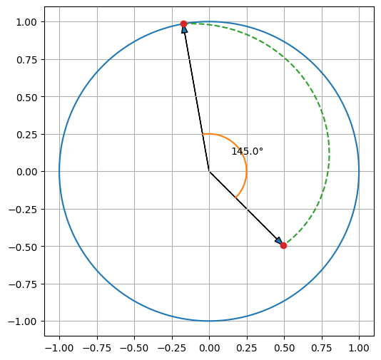
To achieve smooth interpolation between wavetables, the interpolation is done per bin in the frequency domain: for each FFT bin we adjust magnitude and phase linearly, moving phase in the direction of the smallest change.

Step 6
Smooth + play back
We interpolate between wavetables smoothly to avoid discontinuities, then play the result back using WebAudio.
Wavetable player
Audio playback is available in the browser.
Playback uses a shared AudioContext and an AudioWorklet for real-time playback.
Presets + sequencer
We define three sound presets (each with its own color), then use a simple 4-beat piano-roll sequencer (16th-note grid) to draw patterns and play them back in a loop.
Step 7
Presets + sequencer
Implementation
Step 7
Presets + sequencer
Sequencer playback is available in the browser.
Playback uses an AudioWorklet with 5-voice polyphony at 120 BPM.