Original post date: January 9, 2026

GitHub
About this post

After writing this post, I noticed it got quite technical. If you're not into math notation or the like, I hope you can still get something out of it by skimming through the steps and checking out the simulations.

Self-Evolving Cellular Automata

SimulationsProgrammingEmergence

This post started from thoughts about the question of how entropy always increases in an isolated system can still be compatible with locally concentrated, structured patterns. I have a bunch of thoughts on this topic that I might write about at some other time, but they served as inspiration for this implementation of a Game of Life -type simulation.

The main idea was to first make a linear system, where entropy increases over time in a very intuitive way. Then, by introducing nonlinearities and randomness, complexity starts to arise seemingly from nowhere. The starting point is a blend between numerical simulations similar to FDTD and cellular automata (like Conway's Game of Life).

Cell layout diagram
Cell indexing from the perspective of the cell in the center

Step 1

Mechanism with increasing entropy

We start with a grid of cells, which are updated in steps.

All cells are computed in parallel, but let's look at the progression from the perspective of a single cell, which we'll call the focal cell for clarity. Each cell interacts with its 8 immediate neighbors, forming a group of 9. We'll index the cells according to the image to the left.

At each step tt for the focal cell (index 1) we have two important variables: a non-negative energy scalar E1(t)R+E_1^{(t)}\in\mathbb{R}_+ and a transfer matrix W1(t)R9×9.\mathbf{W}_1^{(t)}\in\mathbb{R}^{9\times 9}.

The transfer matrix W1(t)\mathbf{W}_1^{(t)} defines how energy spreads from the cell to its neighborhood. To calculate the spread, the 9 values of all adjacent cells are stacked into a vector e(t)\mathbf{e}^{(t)}, where each entry corresponds to one neighborhood position k.k. The relative spread from the focal cell to all 9 cells in the neighborhood is then calculated according to:

s~1(t)=W1(t)e(t)+ϵ\tilde{\mathbf{s}}_1^{(t)} = \mathbf{W}_1^{(t)}\,\mathbf{e}^{(t)} + \epsilon

We add a very small epsilon to account for situations where the spread would be all zeros - the spread will then be uniform instead. In this first step, we leave the spread like this, noting that the transfer matrix would need to be constrained to positive values, W1(t)R+W_1^{(t)}\in\mathbb{R}_+, to avoid "negative spread of energy".

To compute how the energy is redistributed from the focal cell to the neighborhood while the total energy remains constant, we turn the spread s~1(t)\tilde{\mathbf{s}}_1^{(t)} into a probability-like proportion vector p(t)\mathbf{p}^{(t)} by normalizing it, and then we multiply by E1(t)E_1^{(t)} to obtain the neighborhood energy vector at the next time step e(t+1)\mathbf{e}^{(t+1)}:

p(t)=s~1(t)j=19s~j(t),e1(t+1)=E1(t)p(t).\mathbf{p}^{(t)} = \frac{\tilde{\mathbf{s}}_1^{(t)}}{\sum_{j=1}^{9} \tilde{s}_j^{(t)}},\qquad \mathbf{e}_1^{(t+1)} = E_1^{(t)}\,\mathbf{p}^{(t)}.

When this is done in parallel for all cells in the grid, taking into account things like energy not spreading into certain cells (e.g. walls), we then sum all of these together to get the energy in the whole grid for the next time step.

When energy flows from one cell to another, we also assume that the mechanism of that cell flows with it. For the next time step, the transfer matrix is thus also updated. Let's also consider that from the perspective of the focal cell.

The transfer matrix update is proportional to the energy flow: if no energy were flowing to the focal cell from any other cell except the focal cell itself, the transfer matrix would not change. But since energy will also be flowing in from other cells in varying amounts, we weight all of the neighboring transfer matrices relative to the energy flow as follows:

W~1(t+1)=j=19(ej1(t))2Wj(t)j=19(ej1(t))2+ϵ\begin{aligned} \tilde{\mathbf{W}}_1^{(t+1)} &= \frac{\sum_{j=1}^{9} \left(\mathbf{e}_{j\to 1}^{(t)}\right)^2\,\mathbf{W}_j^{(t)}}{\sum_{j=1}^{9} \left(\mathbf{e}_{j\to 1}^{(t)}\right)^2 + \epsilon} \end{aligned}

We square the energy when weighting, which puts a lot of weight on directions with higher energy flow (note: you do get interesting results also with other powers than 2 here). We again add a small epsilon to account for situations where the energy might be zero.

So, the one thing remaining before we can take our first steps is to figure out how we initialize EE and W\mathbf{W}. Let's initialize W\mathbf{W} at random with positive values and put a chunk of energy in the middle.

Paused Step 0

Even though we initialized the weights with random values, when the energy starts flowing and the weights affect each other, the simulation very quickly stabilizes into a kind of numerical diffusion model. As one might expect with diffusion, over time, it leads to the energy being evenly spread throughout the container.

Step 2

Bringing in randomness

It's perhaps not that surprising that the previous simulation quickly started converging towards a stable solution. We basically had a completely sealed container where we introduce a bunch of energy and allow it to spread out with no constraints or outside influences whatsoever.

Again, let's look at this from the perspective of a single cell, the focal cell.

In the previous step, the mechanism was defined by energy flow; the mechanisms flow with energy. But what if the cell has no energy at all?

If the cell had no energy, it would make sense to define the mechanism as random. But the more energy a cell has, the more the mechanisms will be carried by that energy, and the less this randomness would be.

I'm sure there are other ways to define this, but I chose to define it as follows:

W1(t+1)=λ1(t+1)W~1(t+1)+βξ(1λ1(t+1)),ξN(0,1)\mathbf{W}_1^{(t+1)} = \lambda_1^{(t+1)}\,\tilde{\mathbf{W}}_1^{(t+1)} + \beta\,\boldsymbol{\xi}\,\left(1-\lambda_1^{(t+1)}\right),\qquad \boldsymbol{\xi}\sim\mathcal{N}(0,1) λ1(t+1)=E1(t+1)β+E1(t+1)\lambda_1^{(t+1)} = \frac{E_1^{(t+1)}}{\beta + E_1^{(t+1)}}

It might look a bit complex, but we are essentially just adding randomness whose strength decreases as the energy of the cell increases.

Here W~1(t+1)\tilde{\mathbf{W}}_1^{(t+1)} is the weighted-average transfer matrix from the previous step (computed from incoming energy flows into the focal cell). We then form the next transfer matrix W1(t+1)\mathbf{W}_1^{(t+1)} by blending it with random noise. β\beta sets the overall noise scale, ξ\boldsymbol{\xi} is an elementwise standard normal noise matrix.

So, let's add some randomness to see what it looks like:

Paused Step 0

The result resembles boiling. Interestingly, it also leads to the energy piling up at the corners over time.

Step 3

Adding nonlinearities

This is where nonlinear effects start to dominate.

We're still looking at things from the perspective of a single cell (the focal cell).

Let's introduce a new vector, b\mathbf{b}, in addition to the transfer matrix W\mathbf{W}. You could pretty much say it is part of the transfer matrix, since we'll make it behave identically in many ways: it will flow with the energy, it will be weighted and updated in the same way. This turns the transformation into an affine transformation.

Note that in the previous step the transfer matrix was assumed to stay positive. Here it's actually important that we remove that constraint and allow it to change freely.

We feed the transformation through an arbitrary nonlinear function f.f.:

z1(t)=W1(t)e(t)+b1(t),s1(t)=f ⁣(z1(t))+ϵ.\begin{aligned} \mathbf{z}_1^{(t)} &= \mathbf{W}_1^{(t)}\,\mathbf{e}^{(t)} + \mathbf{b}_1^{(t)}, \\ \mathbf{s}_1^{(t)} &= f\!\left(\mathbf{z}_1^{(t)}\right) + \epsilon. \end{aligned}

This may look familiar if you've seen neural-network style transformations. This part is heavily inspired by neural networks. I've tried a bunch of different nonlinearities (activation functions) here. I got the best results by omitting all negative values (rectified linearity) or feeding it through a step-function (positive values giving the value 1, and other values giving the value 0). Here, we use rectified linearity:

f(x)=max(0,x)f(x)=\max(0,x)

Let's try out the same thing with our nonlinear transformations:

Paused Step 0

In practice, this produces "mechanisms" that appear as the energy spreads. If you reset the simulation a few times, you'll notice different structures forming now and then, sometimes resembling small organisms moving around the grid.

Step 4

More nonlinear features

I made a few additional changes that introduce a wider range of behaviors.

  • I tried adding a little bit of energy everywhere at each time step
  • The energy is also slowly dissipated, to avoid too much energy building up
  • The randomness is applied locally, not uniformly in the simulation
Paused Step 0

The slider controls where the randomness is applied. You'll notice that new mechanisms primarily form where randomness is introduced, and quickly spread out to the area where there is no randomness.

Python simulation screenshot
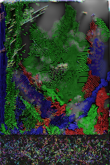
The Python version after having run about 3k steps

When the mechanisms spread, they automatically start "competing" with each other, since the mechanisms that effectively gather the most energy to occupy the cells will remain and replace the ones that are less effective. Every now and then, these mechanisms can be quite complex. This is less apparent in this small simulation than in the complete Python one.

Hosted on GitHub is a repository with the Python script I used to test the ideas outlined on this page, along with a bunch of additional stuff as well. You get a lot more complexity by running this with multiple parallel channels instead of just one, as I do here. It's all there in the repository. I included a very minimal version of the script as well, which is more closely aligned with the version I run on this page.


← Back to blog index